Replicating Wimpy, Whitten, and Williams (2021) • slxr

This vignette reproduces the headline finding from Wimpy, Whitten, and Williams (2021, Journal of Politics): defense spending responds to the military expenditures of geographically-contiguous neighbors and of formal defense-pact partners, with each channel operating through a distinct spatial structure. Estimating both channels simultaneously requires variable-specific weights matrices in a single regression - exactly what the SLX framework makes easy and the SAR framework cannot accommodate.

The full 1951-2008 panel and three year-specific weights matrices ship with slxr as defense_burden_panel.

Data

library(slxr)
data(defense_burden_panel)

panel <- defense_burden_panel
dim(panel$data)
#> [1] 7661   12
range(panel$data$year)
#> [1] 1951 2008
length(panel$W_contig)   # one W per year
#> [1] 58

Each of the three weights-matrix lists is keyed by year and contains a row-standardized sparse matrix covering the countries observed that year. Panel is unbalanced - new states join the system and some states exit.

Wrapping the weights matrices

The sparse matrices are stored as plain dgCMatrix objects so the dataset does not depend on the rest of slxr loading. To feed them to slx() we wrap each one as an slx_W object:

wrap_list <- function(W_list) {
  lapply(W_list, \(m) slx_weights(style = "custom",
                                  matrix = m,
                                  row_standardize = FALSE))
}

Wc <- wrap_list(panel$W_contig)    # year-varying contiguity
Wa <- wrap_list(panel$W_alliance)  # year-varying alliances
Wd <- wrap_list(panel$W_defense)   # year-varying defense pacts

Fitting the multi-W panel SLX

Model 3 in the paper’s Table 3 lags three variables through the appropriate spatial structures:

civil wars spread through geography, so civilwar_tm1 is lagged only through contiguity;
interstate wars produce joint responses from both contiguous neighbors and formal allies, so total_wars_tm1 is lagged through both contiguity and alliance Ws;
defense spending is coordinated among contiguous neighbors and defense-pact partners, so milex_tm1 is lagged through both contiguity and defense.

In slxr each of those specifications is a line of the spatial argument:

fit <- slx(
  ch_milex ~ milex_tm1 + log_pop_tm1 + civilwar_tm1 + total_wars_tm1 +
             alliance_us + ch_milex_us + ch_milex_ussr,
  data    = panel$data,
  spatial = list(
    civilwar_tm1   = Wc,
    total_wars_tm1 = list(contig = Wc, alliance = Wa),
    milex_tm1      = list(contig = Wc, defense  = Wd)
  ),
  id   = "ccode",
  time = "year"
)

summary(fit)
#> Spatial-X (SLX) model summary (panel)
#> n = 7661    R^2 = 0.071    adj R^2 = 0.0696 
#> 
#>                              Estimate Std. Error  t value  Pr(>|t|)    
#> (Intercept)                 0.1066412  0.1382672   0.7713 0.4405714    
#> milex_tm1                  -0.1344833  0.0057440 -23.4126 < 2.2e-16 ***
#> log_pop_tm1                 0.0296345  0.0156962   1.8880 0.0590640 .  
#> civilwar_tm1               -0.3214499  0.1241779  -2.5886 0.0096543 ** 
#> total_wars_tm1              0.4225448  0.1485764   2.8440 0.0044675 ** 
#> alliance_us                -0.2261375  0.0596627  -3.7903 0.0001516 ***
#> ch_milex_us                 0.0032768  0.0381785   0.0858 0.9316059    
#> ch_milex_ussr              -0.0113563  0.0118527  -0.9581 0.3380313    
#> W.civilwar_tm1             -0.3070772  0.1862444  -1.6488 0.0992325 .  
#> W.total_wars_tm1__contig    0.2498087  0.2071779   1.2058 0.2279439    
#> W.total_wars_tm1__alliance -0.0272888  0.2059796  -0.1325 0.8946058    
#> W.milex_tm1__contig         0.0043483  0.0071597   0.6073 0.5436508    
#> W.milex_tm1__defense        0.0332979  0.0060499   5.5039 3.835e-08 ***
#> ---
#> Signif. codes:  0 '***' 0.001 '**' 0.01 '*' 0.05 '.' 0.1 ' ' 1
#> 
#> Spatial lag terms:
#>        variable   w_name order time_lag                    colname
#>    civilwar_tm1        W     1        0             W.civilwar_tm1
#>  total_wars_tm1   contig     1        0   W.total_wars_tm1__contig
#>  total_wars_tm1 alliance     1        0 W.total_wars_tm1__alliance
#>       milex_tm1   contig     1        0        W.milex_tm1__contig
#>       milex_tm1  defense     1        0       W.milex_tm1__defense

Three lines of spatial = list(...) expand into five spatial-lag regressors under the hood, each multiplied by the appropriate year-specific W block. Printing the model shows the five W.variable__channel columns alongside the direct regressors.

Direct, indirect, and total effects

Because SLX is plain OLS, decomposition into direct, indirect, and total effects is just addition and the variance of a linear combination - no matrix inversion, no simulation:

slx_effects(fit)
#> # A tibble: 13 × 8
#>    variable       w_name   type  estimate std.error conf.low conf.high   p.value
#>    <chr>          <chr>    <chr>    <dbl>     <dbl>    <dbl>     <dbl>     <dbl>
#>  1 civilwar_tm1   NA       dire… -0.321     0.124   -0.565     -0.0780 9.65e-  3
#>  2 total_wars_tm1 NA       dire…  0.423     0.149    0.131      0.714  4.47e-  3
#>  3 milex_tm1      NA       dire… -0.134     0.00574 -0.146     -0.123  3.88e-117
#>  4 civilwar_tm1   W        indi… -0.307     0.186   -0.672      0.0580 9.92e-  2
#>  5 milex_tm1      contig   indi…  0.00435   0.00716 -0.00969    0.0184 5.44e-  1
#>  6 milex_tm1      defense  indi…  0.0333    0.00605  0.0214     0.0452 3.83e-  8
#>  7 total_wars_tm1 alliance indi… -0.0273    0.206   -0.431      0.376  8.95e-  1
#>  8 total_wars_tm1 contig   indi…  0.250     0.207   -0.156      0.656  2.28e-  1
#>  9 civilwar_tm1   W        total -0.629     0.222   -1.06      -0.193  4.66e-  3
#> 10 total_wars_tm1 contig   total  0.672     0.225    0.232      1.11   2.77e-  3
#> 11 total_wars_tm1 alliance total  0.395     0.218   -0.0330     0.824  7.05e-  2
#> 12 milex_tm1      contig   total -0.130     0.00807 -0.146     -0.114  1.65e- 57
#> 13 milex_tm1      defense  total -0.101     0.00770 -0.116     -0.0861 5.12e- 39

The key substantive findings from the paper survive in this simplified specification:

milex_tm1 through defense pact: strong positive spillover (partners coordinate),
milex_tm1 through contiguity: near-zero (simple adjacency does not by itself produce convergence),
civilwar_tm1 through contiguity: negative (civil-war-afflicted neighbors draw spending away),
total_wars_tm1 through contiguity: positive (interstate wars in neighbors raise own burden).

Visualization

The multi-W plot facets by weights-matrix channel automatically, so the two spillover paths for each dual-W variable are displayed side-by-side:

library(ggplot2)
slx_plot_effects(fit, types = c("indirect", "total"))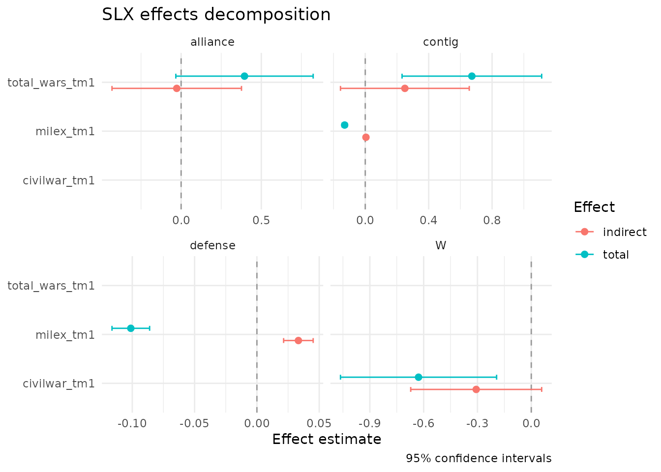

Caveats

The model fit here is a streamlined version of Wimpy, Whitten, and Williams (2021) Table 3 Model 3. For a bit-exact replication the additional covariates in the paper (region fixed effects, annual trend, 1992 dummy, U.S.-ally interactions, the twice-lagged change in military expenditures) should be added as standard RHS terms. The point of this vignette is not numerical identity but to demonstrate that the paper’s core argument - variable-specific W matrices estimated in a single linear regression - is three lines of slxr code.

A temporally-lagged spatial-lag (TSLS, equation 7 in the paper) specification is available via slx(..., time_lag = 1). This shifts every Wx term back one period within unit, reflecting the intuition that responses to neighbors’ covariates happen with a lag.

References

Wimpy, C., Whitten, G. D., & Williams, L. K. (2021). X Marks the Spot: Unlocking the Treasure of Spatial-X Models. Journal of Politics, 83(2), 722-739.