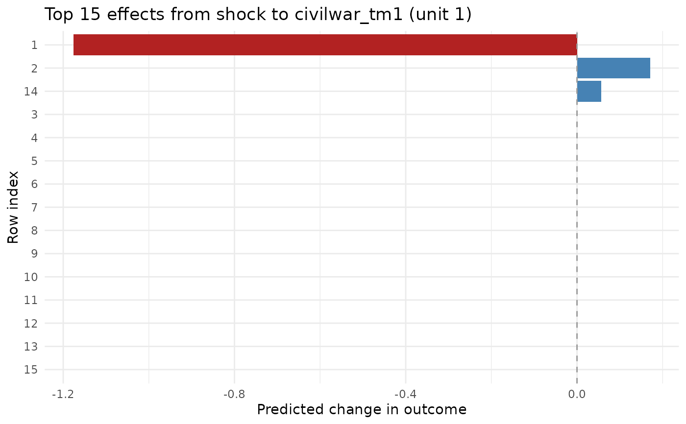
Given a fitted SLX model, a choice of variable, and a target unit, returns a plot of the predicted change in the outcome across every unit in the sample under a unit shock to that variable in the target unit.
Arguments
- fit
A cross-sectional
slxmodel. Panel shocks are planned for a future release.- variable
Character, the name of a spatially-lagged regressor in
fitto shock.- unit
Integer row index (or character id, if the weights matrix has dimnames matching something in
fit$data) of the unit receiving the shock.- magnitude
Numeric, shock size. Default
1.- geom
Optional
sfobject withnrow(geom) == fit$naligned tofit$data. If supplied, the function returns a map.- top_n
For the non-map plot, how many non-zero indirect effects to show. Default
15.
Details
For an SLX model at first order with channels indexed by c, the
predicted change at unit j from a shock of size magnitude to
variable x in unit i is
$$\text{magnitude}\ \left(\beta\ \mathbb{1}\{j=i\} + \sum_c \theta_c\ W_c[j, i]\right).$$
Higher-order lags add additional theta_{c,k} (W_c^k)[j, i] terms.
No simulation is required: the shock effect is a single column of
the spatial multiplier.
If an sf object with matching row count is supplied via geom,
the result is drawn as a choropleth. Otherwise a horizontal bar of
the largest effects is returned.
Examples
data(defense_burden)
W_c <- slx_weights(style = "custom", matrix = defense_burden$W_contig,
                   row_standardize = FALSE)
fit <- slx(ch_milex ~ milex_tm1 + civilwar_tm1,
           data = defense_burden$data, W = W_c,
           lag = "civilwar_tm1")
slx_plot_shock(fit, variable = "civilwar_tm1", unit = 1)